From Static Lexicons to Dynamic Context: How Word2Vec Revolutionized NLP

Overcoming WordNet's Rigidity and One-Hot Encoding's Sparsity with Distributional Semantics

Language, as a dynamic social system, evolves through human interaction, cultural shifts, and contextual nuance, presenting unique challenges for computational interpretation. Traditional methods, such as lexical databases (e.g., WordNet) and one-hot encoding, treated words as static or isolated symbols, failing to capture semantic relationships.

WordNet:

WordNet is essentially a lexical database for English. A lexical database is essentially a structured resource that stores & organizes information with regards to words, their meanings, relationships and usage in a language.

import nltk
nltk.download('wordnet')
from nltk.corpus import wordnet as wn

word = "car"

# Get all synsets (semantic groupings) for the word
synsets = wn.synsets(word)
print("Synsets for 'car':", [syn.name() for syn in synsets])

# Get synonyms (lemmas) for the first synset
first_syn = synsets[0]
print("\nFirst synset:", first_syn.name())
print("Definition:", first_syn.definition())
print("Synonyms:", [lemma.name() for lemma in first_syn.lemmas()])

# Get hypernyms (more general categories)
hypernyms = first_syn.hypernyms()
print("\nHypernyms:", [hyp.name() for hyp in hypernyms])

hyponyms = first_syn.hyponyms()
print("\nHyponyms:", [hyp.name() for hyp in hyponyms])

meronyms = first_syn.part_meronyms()
print("\nMeronyms:", [mer.name() for mer in meronyms])

Output:

Synsets for 'car': ['car.n.01', 'car.n.02', 'car.n.03', 'car.n.04', 'cable_car.n.01']

First synset: car.n.01
Definition: a motor vehicle with four wheels; usually propelled by an internal combustion engine
Synonyms: ['car', 'auto', 'automobile', 'machine', 'motorcar']

Hypernyms: ['motor_vehicle.n.01']

Hyponyms: ['roadster.n.01', 'convertible.n.01', 'subcompact.n.01', 'touring_car.n.01', 'gas_guzzler.n.01', 'beach_wagon.n.01', 'coupe.n.01', 'pace_car.n.01', 'stanley_steamer.n.01', 'jeep.n.01', 'electric.n.01', 'loaner.n.02', 'minicar.n.01', 'hot_rod.n.01', 'compact.n.03', 'cruiser.n.01', 'hatchback.n.01', 'sedan.n.01', 'sports_car.n.01', 'hardtop.n.01', 'stock_car.n.01', 'model_t.n.01', 'cab.n.03', 'racer.n.02', 'minivan.n.01', 'limousine.n.01', 'used-car.n.01', 'bus.n.04', 'sport_utility.n.01', 'horseless_carriage.n.01', 'ambulance.n.01']

Meronyms: ['car_door.n.01', 'reverse.n.02', 'bumper.n.02', 'car_seat.n.01', 'high_gear.n.01', 'third_gear.n.01', 'window.n.02', 'tail_fin.n.02', 'running_board.n.01', 'air_bag.n.01', 'hood.n.09', 'luggage_compartment.n.01', 'automobile_engine.n.01', 'roof.n.02', 'auto_accessory.n.01', 'gasoline_engine.n.01', 'sunroof.n.01', 'automobile_horn.n.01', 'fender.n.01', 'buffer.n.06', 'rear_window.n.01', 'floorboard.n.02', 'glove_compartment.n.01', 'car_window.n.01', 'grille.n.02', 'accelerator.n.01', 'first_gear.n.01', 'car_mirror.n.01', 'stabilizer_bar.n.01']

synsets - short for synonyms set that groups together words that have similar meanings.

semantics - study of meaning in a language

lemma - base or dictionary form of a word

hypernyms - word or phrase that denotes general category of object, concepts or entities (motor vehicle for car)

hyponyms - word or phrase that denotes specific concept within a broader category represented by hypernyms (convertible for car )

meronyms - word or phrase that denote a part or component of a larger whole. In other words, meronyms represents relationship where one term is part of another term. (wheel is part of car)

# definition of all synsets of the word car
[synsets[x].definition() for x in range(len(synsets))]
['a motor vehicle with four wheels; usually propelled by an internal combustion engine', 'a wheeled vehicle adapted to the rails of railroad', 'the compartment that is suspended from an airship and that carries personnel and the cargo and the power plant', 'where passengers ride up and down', 'a conveyance for passengers or freight on a cable railway']

From the output above, it can be seen that synset definitions for the word car are words that represents similar meaning like motor vehicle, trains, etc.

Where does WordNet fall short? While it was a good step forward in modeling language computationally, there were couple of major limitations:

1. There was a lack of context sensitivity where WordNet treats words as static entities with fixed synsets (eg. “bank” as financial intuition vs. a riverbank). This led to failure to resolve ploysemy (multiple word meanings) in a context. Here is another example - “Apple company vs. fruit OR my car was broken, great vs. food was great!”

2. It is manually created and hence slow to update. Also, not comprehensive. It may not incorporate evolving languages and modern slangs.

3. It has limited language coverage where most of the focus is on English language with sparse support for other languages. As a result, there is limited multi-language application.

4. There is no quantitative way to measure the semantic relationship. WordNet provides hierarchical relationships of words in terms of hypernyms and hyponymns but lacks semantic similarity metrics. How to quantitatively represent that ‘dog is closer to puppy than a lion’?

One-Hot Encoding:

This is pretty widely used techniques especially in traditional machine learning setting where categorical variables are converted into binary metrics. In context of words, it converts words into sparse vectors where each word is orthogonal.

# word tokenizer (one hot encoded)


from sklearn.preprocessing import LabelEncoder, OneHotEncoder
import numpy as np

# Sample corpus
corpus = ["the cat sat on the mat", "the dog ate the food"]

# Tokenize and create vocabulary
tokens = [sentence.split() for sentence in corpus]
vocab = set(word for sentence in tokens for word in sentence)
vocab = sorted(vocab)  # Ensure consistent order
vocab_size = len(vocab)

# Map words to indices
label_encoder = LabelEncoder()
integer_encoded = label_encoder.fit_transform(vocab)

# One-hot encode
onehot_encoder = OneHotEncoder(sparse_output=False)
onehot_encoded = onehot_encoder.fit_transform(integer_encoded.reshape(-1, 1))

# Create a word-to-one-hot dictionary
word_to_onehot = {word: vec for word, vec in zip(vocab, onehot_encoded)}

# Example: One-hot vector for "cat"
print("One-hot for 'cat':", word_to_onehot["cat"])

Output:

>>> word_to_onehot
{'ate': array([1., 0., 0., 0., 0., 0., 0., 0.]), 'cat': array([0., 1., 0., 0., 0., 0., 0., 0.]), 'dog': array([0., 0., 1., 0., 0., 0., 0., 0.]), 'food': array([0., 0., 0., 1., 0., 0., 0., 0.]), 'mat': array([0., 0., 0., 0., 1., 0., 0., 0.]), 'on': array([0., 0., 0., 0., 0., 1., 0., 0.]), 'sat': array([0., 0., 0., 0., 0., 0., 1., 0.]), 'the': array([0., 0., 0., 0., 0., 0., 0., 1.])}

# sentence tokenizer (one hot encoded)

from tensorflow.keras.preprocessing.text import Tokenizer
# Initialize tokenizer
tokenizer = Tokenizer()
tokenizer.fit_on_texts(corpus)

# Convert text to integer sequences
sequences = tokenizer.texts_to_sequences(corpus)

# Convert integers to one-hot encoding
onehot_results = tokenizer.texts_to_matrix(corpus, mode='binary')

print("Vocabulary:", tokenizer.word_index)
print("One-hot for first sentence:\n", onehot_results[0])

Output:

>>> print("Vocabulary:", tokenizer.word_index)
Vocabulary: {'the': 1, 'cat': 2, 'sat': 3, 'on': 4, 'mat': 5, 'dog': 6, 'ate': 7, 'food': 8}
>>> print("One-hot for first sentence:\n", onehot_results[0])
One-hot for first sentence:
 [0. 1. 1. 1. 1. 1. 0. 0. 0.]

Limitations to represents texts using one-hot encoding is actually quite a bit. First, one hot encoding is not scalable. As the corpus grow, the dimensions grows proportionally which makes it computationally inefficient and is prone to case curse of dimensionality. Additionally, there is no semantic relationship between words as it treats each word as orthogonal. The technique is also context agnostic as same word always maps to the same vector.

This limitation spurred the adoption of distributional semantics, which posits that meaning emerges from context—a hypothesis crystallized in Word2Vec (2013).

Word2Vec

Word2Vec is not a singular algorithm. Rather, it is a family of model architectures and optimizations that can be used to learn word embeddings. Word2Vec is developed by Google.

The core concept of Word2Vec is that a word's meaning is determined by the words that commonly appear near it—a highly influential idea in NLP. For example, "dog" and "puppy" often appear near words like "bark," "leash," or "pet," so their embeddings (vector representations) will be geometrically close in the learned vector space. By training neural networks to predict word co-occurrences, Word2Vec generated dense vector embeddings where geometric proximity reflects semantic similarity (e.g., "king" – "man" + "woman" ≈ "queen").

Essentially, Word2Vec trains a shallow neural network to create word representations:

The input for word2Vec contains all documents/texts in the training set. For neurons to process the texts, they are represented in the one-hot encoding of the words. The number of neurons present in the hidden layer is equal to the number of embedding we want. In order words, if we want all our words to be vectors then the hidden layer will contain 300 neurons.

At the end of the training, the hidden weights are treated as word embeddings. Intuitively, this can be thought of as each word having set of n weights (300 weights assuming hidden layer has 300 neurons)

In the figure above, a input of 10,000 corpus is passed to the neural network. The input to the model is one-hot encoded vector with one element set to 1 and the rest 0. The hidden layer consists of a weight matrix of 10,000 * 300. Each row in this matrix represents the word in the vocabulary and 300 columns represents embedding dimensions. Finally, after training, the hidden layer’s weight matrix serves as a look up table for word embeddings. For each word, the corresponding row in the weight matrix is 300-dimensional vector representation.

Why 300 features instead of 1000?

• Dimensionality Reduction: The 300 features are a compressed representation of each word, capturing its essential semantic properties in a lower-dimensional space.

• Efficiency: A 10,000-dimensional representation would be computationally expensive and redundant, while 300 dimensions strike a balance between efficiency and expressive power.

• Semantic Relationships: The 300-dimensional space allows words with similar meanings to have embeddings that are close to each other, capturing patterns like "king - man + woman = queen."

Intuitively, think of weight matrix as a transformation from a sparse, high dimensional one hot representation (10,000) dimensions to a dense, meaningful representation (300 dimensions). This is essence of Word2Vec’s ability to learn word representations.

Word2Vec has two training approaches to learn the representations of the word: Skip-gram and Continuous Bag of Words (CBOW).

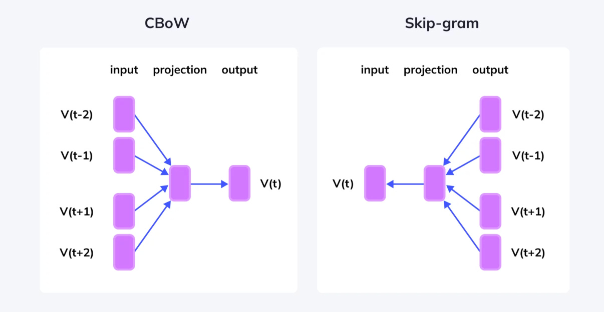
SkipGram: predicts the context words based on the center word. In other words, it predicts words within a certain range before and after the current word in the same sentence.

Continous Bag of Words (CBOW): predicts the center word based on the context word. The architecture is called Bag of Words because the order of words is not important. CBOW allows for faster training and is better for frequent words.

Word2Vec allows you to choose one of the two architectures (Skip-gram or CBOW) for training a model—it does not use both simultaneously.

Practical Advice

1. Skip-gram is often preferred for its ability to handle rare words and nuanced relationships.

2. Use CBOW if:

   • You have a massive corpus and prioritize training speed.

   • Your task benefits from smoothing over context (e.g., topic modeling).

gensim is a popular library in Python for Word2Vec. In gensim library, you specify the architecture via the sg parameter:

• sg=1 → Skip-gram

• sg=0 → CBOW

from gensim.models import Word2Vec

# Skip-gram model
model_sg = Word2Vec(sentences, vector_size=100, window=5, sg=1, min_count=1)

# CBOW model
model_cbow = Word2Vec(sentences, vector_size=100, window=5, sg=0, min_count=1)

Using gensim, pre-trained models on large corpus could be used. One of the model is from Google called word2vec-google-news-300. gensim also allows for creation of custom embeddings. In other words, user created files/corpus can be used for generating embedding which can then be used for other downstream applications.

Another interesting insight about Word2Vec is that it is self supervised learning. Self-supervised learning is a type of supervised learning where the training labels are determined by the input data itself, without the need for manual labeling. Word2Vec uses the context of words in a corpus to generate its own training data.

Here is an example of Word2Vec using skip-gram on a large corpus which contains a wide variety of topics, as it is derived from English Wikipedia. The dataset contains approximately 17 million words after tokenization.

from gensim import downloader
dataset = downloader.load('text8')
sentences = list(dataset)   # input should be a list of tokenized sentences

# Training the Word2Vec model
model = Word2Vec(
    sentences, 
    vector_size=100,  # Embedding dimensions
    window=5,         # Context window size 
    min_count=5,      # Minimum word frequency
    workers=4,        # Number of CPU cores
    sg=1              # Skip-Gram model
)

vector_size → emphasizes how many features each words would have (dimensions). A large vector size captures more semantic relationship but requires more memory and computational power. For vector_size=100, each word will be represented by a 100-dimensional vector, e.g., [0.1, 0.23, ..., -0.12].

window → defines maximum distance between target word and its context word during training.

min_count → ignores all word that appear fewer than min_count times in corpus.

workers → specifies the number of CPU cores to use in parallelization during training.

sg → 0 = CBOW and 1 = skip-gram

---

Exploring Word Embeddings

a) Explore vector of a word:

>>> vector = model.wv['king']  
>>> print(vector)
[ 0.08122083  0.07926018  0.35090202  0.36486888  0.90775234  0.24396007
  0.06873245 -0.14285737 -0.1855695   0.15459074 -0.70231104 -0.39637893
  0.29327387  0.02936908 -0.17457394 -0.01639966  0.35264775 -0.14727874
  0.55718225 -0.12398887 -0.09546658  0.55053234 -0.04490681 -0.12874283
  0.09575947 -0.03059613  0.0073285   0.06962211 -0.2771781   0.3545496
  0.17587571  0.12756832  0.09257357 -0.08313553 -0.01367026  0.08208441
 -0.15594321 -0.28755006 -0.2832372  -0.12549688  0.32955956 -0.19233881
 -0.13212588  0.12642798 -0.07827964 -0.16524078 -1.0867044   0.07889321
  0.81744045 -0.12846221  0.408422   -0.30254152 -0.44793576 -0.0260348
  0.5627293  -0.5491161   0.42907977  0.04579482  0.12987387  0.00301055
  0.34862745  0.2025278   0.38379073 -0.08277258 -0.19507341 -0.1575186
  0.42863113  0.39006442  0.25645357  0.39950788  0.22158371  0.25421777
  0.15680233  0.09712736  0.1323583  -0.01493575  0.34186122  0.231322
 -0.36201417  0.25226715 -0.07077599 -0.60105544 -0.44324198  0.47023138
  0.34849274  0.6353434   0.72335654 -0.0416906   0.19091745  0.29033056
  0.6171756   0.07778944  0.48299393 -0.23152421  0.33724144  0.4522352
  0.27884063  0.10636301 -0.3708287  -0.40318197]

b) Find similar word

>>> similar_words = model.wv.most_similar('king', topn=5)
>>> print(similar_words)
[('prince', 0.7636538147926331), ('canute', 0.7306182980537415), ('valdemar', 0.7299929261207581), ('haakon', 0.7283191680908203), ('queen', 0.7208762764930725)]

c) Find similarity between words

similarity = model.wv.similarity('king', 'queen')
>>> print(f"Similarity between 'king' and 'queen': {similarity}")
Similarity between 'king' and 'queen': 0.7208764553070068 

d) Word Analogy

>>> result = model.wv.most_similar(positive=['king', 'woman'], negative=['man'], topn=1)
>>> print(f"Word closest to 'king - man + woman': {result}")
Word closest to 'king - man + woman': [('queen', 0.6826784610748291)]

The word embedding can be further fine tuned if provided additional datasets.

These word embeddings can be visualized. In the future posts, I will explore the dimensionality reduction techniques like PCA and t-SNE. Using t-SNE, the following is the first 100 words of the embeddings visualized:

As can be seen, the word ‘united’ and ‘states’ are very close to one another in the vector space. Another interesting one is ‘world’ and ‘war’ which It would be fine if they were not so close together :(

Final things to note is that negative sampling and hierarchical soft max are two alternatives used in Word2Vec to efficiently compute probabilities on a large vocabulary. Both address the challenge of training models on datasets with millions of words by approximating the computationally expensive softmax function.

Negative Sampling → Instead of calculating probability distribution over all words in the vocabulary, negative sampling focuses on updating only the small subsets of words during training.

Hierarchical softmax → replaces the softmax function with a binary tree structure to approximate the probability distribution over the vocabulary.

While Negative Sampling is often used while training a large corpus, Hierarchical softmax is mostly used for smaller vocabularies or training with limited resources.

---

References:

https://medium.com/@manansuri/a-dummys-guide-to-word2vec-456444f3c673