Graph Fundamentals and Their Role in Machine Learning

Understanding graph structures, representations, and traditional feature engineering techniques for modeling complex relational data

Graphs are a universal language to represent entities (nodes) and their relationships (edges). As the need to model complex interactions grows, graphs are becoming increasingly popular across domains, from social networks to recommendation engines, because they naturally represent relational structure.

A graph G is formally defined as an ordered pair:

where V is set of vertices (nodes) representing entities and E which is subset of V * V is set of edges (links) representing the relationship between pair of nodes.

Why Graphs for modeling?

Traditional machine learning models are designed for grid-like (Euclidean) data such as images or text. However, many real-world systems are better described as non-Euclidean structures such as irregular, unordered, and relational. Graphs fill this gap, enabling us to capture intricate dependencies between entities that traditional models fail to represent effectively.

Common Examples of Graphs

• Citation networks: Papers as nodes, citations as edges

• Social networks: Users as nodes, friendships or follows as edges

• Knowledge graphs: Entities as nodes, relationships as typed edges

Types of Graphs

• Directed vs. Undirected Graphs: Represent asymmetric or symmetric relationships

• Weighted Graphs: Edges carry weights (e.g., distances, scores)

• Heterogeneous Graphs: Multiple types of nodes or edges (e.g., user-item graphs in recommendation systems)

• Line Graphs and Planar Graphs: Specialized graph structures with specific topological constraints

• Unweighted Graphs: Edges do not carry weights and just indicate presence or absence of connection

• Self loops - Nodes can have edges pointing to themselves

• Multigraph - Allows multiples graphs between the same pair of nodes (i.e multiple edges can exist between same pair of nodes)

Challenges in Graph Modeling

Graph data is non-Euclidean, irregular, and often dynamic. Graphs can:

• Vary in size

• Have no fixed node ordering

• Exhibit complex topology and spatial locality

• Contain multimodal or time-evolving features

This complexity makes applying standard deep learning techniques non-trivial, requiring dedicated architectures like Graph Neural Networks (GNNs).

Core Graph Modeling Tasks

• Node-Level Tasks

  • Node Classification: Predict labels for individual nodes (e.g., user roles, fraud detection)

  • Node Clustering: Group nodes based on similarity or connectivity

• Edge-Level Tasks

  • Link Prediction: Predict whether an edge exists between two nodes (e.g., friend suggestion, missing facts in knowledge graphs)

• Graph-Level Tasks

  • Graph Classification: Predict labels for entire graphs (e.g., molecule toxicity, document topic)

  • Graph Generation: Create new graphs (e.g., drug discovery, scene generation)

• Subgraph-Level (Community-Level) Tasks

  • Community Detection: Identify clusters or communities within a graph

Key Concepts in Graph Modeling

How to define the graph?

• What entities are nodes?

• What relationships are edges?

• Should the graph be directed, undirected, weighted, or heterogeneous?

Choosing the right graph representation directly impacts model performance and interpretability.

Important Concepts

Node degree - represents the number of neighbors in a node. For directed graph, there is in-degree and out-degree. The total degree is sum of in and out degrees.

Bipartite Graph - Bipartite graph is a graph where nodes can be divided into 2 disjoint sets U and V such that every link connects a node in U to on in V.

Adjacency matrix: The adjacency matrix is a standard way to represent a graph in matrix form.

For weighted graphs, A[i][j] = weight from the edge i to j

For unweighted graph, A[i][j] = 1 or 0

For undirected graph → A is symmetric and for directed graph → A is asymmetric.

Representing graphs in matrix form enables algebraic operations for modeling. While adjacency matrix are useful, it is not memory efficient.

In most real world networks networks, each node connects to only a small subset of other nodes. As a result their adjacency matrix are sparse (filled with mostly zeros).

This means that there should be a better way to represent would be to use adjacency list! The following compares various graph representation methods and their pros and cons:

Edge List: A straightforward representation that stores all edges as pairs, e.g., (u1,v1), (u2,v2)…. Suitable for small graphs or simple graph construction. However, it lacks efficient support for quickly retrieving a node’s neighbors.

Adjacency Matrix: Ideal for dense graphs and well-suited for performing matrix operations. However, it is not memory-efficient, especially for sparse graphs, as it stores many zero entries.

Adjacency list: Represents each node alongside its list of neighbors. It is well-suited for large, sparse networks. Advantages include memory efficiency (since zeros are not stored), quick access to a node's neighbors, and ease of edge iteration.

Furthermore, nodes and edges carry additional information beyond just connectivity. These attributes enrich the graph and are crucial in modeling tasks.

Common Node & Edge Attributes

1. Weight

   • Quantifies strength or frequency of interaction.

   • Example: Number of messages between users.

2. Ranking

   • Indicates ordered relationships.

   • Example: Best friend vs. second-best friend.

3. Type

   • Used in heterogeneous graphs to distinguish different kinds of nodes or edges.

   • Example: User, Item, Review; or Friend, Purchaser, Viewer.

4. Sign

   • Encodes positive or negative relationships.

   • Example: Trust vs. distrust; like vs. dislike.

5. Structural Properties

   • Attributes derived from the overall graph structure.

   • Example: Node centrality, clustering coefficient, PageRank score.

Connectivity in Graphs

Connectivity basically formalizes how nodes in the graph are linked together through edges.

1. Undirected Graphs

• Connected Graph:
  Every pair of vertices has at least one path connecting them.

• Disconnected Graph:
  Consists of two or more connected components. That is, subgraphs where nodes are internally connected but no connections exist between components.

• Adjacency Matrix for Disconnected Graphs:
  Can be arranged in a block diagonal form, where each block corresponds to a connected component.
  Non-zero elements appear only inside these blocks, and zeros fill the off-block regions.

2. Directed Graphs

• Strongly Connected Graph:
  For every pair of nodes u and v, there is a directed path from u to v and from v to u.

• Weakly Connected Graph:
  The graph is connected if you ignore the direction of edges (treat all edges as undirected).

• Strongly Connected Components (SCCs):
  Maximal subgraphs where every node is reachable from every other node by following directed edges. Not every node must belong to a non-trivial SCC; some nodes may be isolated or part of trivial SCCs (single nodes).

To summarize above, in an undirected graph, two nodes are considered connected if there is a path between them using the edges. The graph is called connected if every pair of nodes has a path between them. If not all nodes are reachable from each other, the graph is disconnected and consists of multiple connected components. Each component is a group of nodes where all nodes can reach each other, but no connections exist between different components.

For a directed graph, connectivity depends on the direction of edges. A graph is strongly connected if there is a directed path from each node to every other node and vice versa. This means that for any two nodes, both directions are reachable through valid edge paths. A graph is weakly connected if the graph becomes connected when edge directions are ignored, even though some directed paths may be missing. Like undirected graphs, directed graphs can also have disconnected components where some groups of nodes are isolated from others.

Use of graph in Machine Learning

Traditionally, machine learning on graphs relied heavily on manual feature engineering and domain expertise. This was similar to classical ML in other fields that requires manual effort to extract meaningful features from data.

This means:

• Feature Engineering

  • Design and extract meaningful features for the fundamental units:

    • Nodes (e.g., degree, centrality, attributes)

    • Edges/Links (e.g., edge weight, type, frequency)

    • Entire Graphs (e.g., density, clustering coefficient, motifs)

• Feature Extraction

  • Collect these features for all samples in the training dataset (nodes, edges, or whole graphs depending on the task).

• Prediction

  • For any new input (node/link/graph), compute its features using the same process.

  • Feed these features into a trained model to generate predictions (e.g., node classification, link prediction, graph classification).

The following describes mathematical formulation for graph machine learning:

Over time, different levels of feature concepts were introduced to better capture the underlying functions governing graph data.

Feature Levels in Graphs

a. Node-Level Features

The goal of node-level features is to characterize the structure and role of individual nodes within a network, capturing their connectivity, importance, and local structure.

1. Node Degree

• Definition: The number of edges connected to a node.

• Intuition: Measures how many neighbors a node has.

• Limitation: Treats nodes with the same degree equally, ignoring the importance or influence of neighbors.

• Example: In a social network, degree corresponds to how many friends a person has.

2. Node Centrality

• Purpose: Quantify the importance or influence of a node in the graph beyond just counting neighbors.

• Unlike degree, centrality considers the position of the node within the entire network and/or the importance of its neighbors.

• Common types:

  • Eigenvector Centrality: A node is important if it is connected to other important nodes. It is computed as the principal eigenvector of adjacency matrix.

  • Betweenness Centrality: Measures how often a node appears on a shortest paths between other nodes. This captures nodes that serve as a bridge. A high betweenness node can control information flow.

  • Closeness Centrality: Measures the average shortest path distance from a node to all other nodes. Nodes with low average distance are more central (closer to others).

3. Clustering Coefficient

• Measures how well a node’s neighbors are connected to each other. This helps to capture the the nodes to form triangle or cliques locally. High clustering means neighbors are likely to know each other.

4. Graphlets and Mortifs

• Graphlets are small, connected, non-isomorphic induced subgraphs of a larger network. To clarify, non-isomorphic means graphs that are structurally different. Example graphlets include triangles, chains, stars, squares, etc. Motifs are specific graphlets that occur significantly more often in a given network than expected in a random network. Because of this, they reveal important recurring structural patterns that may have functional significance.

  • Graphlets and motifs help characterize the local topology of complex networks.

  • Graphlet Degree Vector (GDV) is a feature vector that captures the local topology around a node by counting how many times it touches each type of small graphlet, in each unique role (called orbits). Orbits represent distinct positions a node can occupy in a graphlet.

To make the idea of GDV more concete, here is an example:

Let’s say we compute GDV using 2–3 node graphlets:

• Orbit 0: Degree (number of direct neighbors)

• Orbit 1: Number of 2-length paths the node is in (middle node in A–B–C)

• Orbit 2: Number of triangles the node is part of

A node with GDV = [3, 2, 1] means:

• It has 3 direct neighbors

• It is the center of two 3-node chains

• It is part of one triangle

In summary, node level features can be categorized into two high level classification:

1. Importance based Features:

   1. Node Degree - counts the number of neighboring node - a node with high number of neighbor → importance

   2. Node Centrality - importance of neighboring nodes

2. Structural Relationship Features:

   1. Node Degree - counts the number of neighboring node - this can specifies local structure of a given node by counting its neighbors

   2. Clustering coefficient - measures how connected neighboring nodes are

   3. GDV - Counts the occurrences of different graphlets.

b. Link level features

Link level features are useful for modeling tasks like predicticing whether a link exists or will form between two nodes in a grpah. Example tasks include recommending friends in social networks, predicting interactions in biological networks, and inferring missing relationship in knowledge graphs. Essentially, the main goal of link-level features is to describe and predict relationships (edges) between pairs of nodes in a graph.

1. Pairwise structural features

• Captures how close two nodes are based on graph topology:

  • Common Neighbors: Number of shared neighbors between nodes

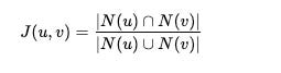
  • Jaccard Coefficient: Ratio of common neighbors between two nodes. It is basically intersection over union.

    

  • Adamic-Adar Index: Sum of inverse logarithmic degrees of common neighbors, giving more weight to less-connected neighbors.

    

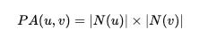
  • Preferential Attachment: Product of degrees of two nodes, based on the idea that high degree nodes tend to connect.

    

2. Path Based Features

• Number or length of paths connecting the two nodes.

• Shorter or multiple paths may indicate higher likelihood of a link.

• Katz index: Measures the connectivity by summing over all possible paths between two nodes, weighting shorter paths more heavily by applying exponential decay factor. It captures both direct and indirect connections, providing richer similarity score. (uses graph’s global structure to calculate)

3. Edge Attributes

• Features such as edge weights, types, or temporal info if the graph is dynamic.

c. Graph Level Features and Graph Kernels

The purpose of graph level features is to describe overall properties and structure of the graph, rather than individual edges or nodes. These features capture global characteristics useful for tasks like graph classification, regression or similarity comparison.

• Number of Nodes

  • Total count of nodes in the graph

  • Indicates graph size

• Number of Edges

  • Total count of edges in the graph

  • Related of graph density

• Graph Density

  • Measures how many edges exist relative to the maximum possible edge

    

• Average Degree

  • Mean number of connections per node

    

• Degree Distribution

  • Statistical distribution of node degrees

  • Can be summarized by moments like mean, variance, and skewness

• Clustering Coefficient (Global)

  • Average of all nodes’ clustering coefficient or ratio of closed triplets to total triplets

  • Indicates tendency of nodes to form clusters

• Diameter

  • The longest shortest path between any two nodes in the graph

  • Reflects the graph’s spread or maximum distance

• Average Shortest Path Length

  • Mean distance between all pairs of nodes

  • Indicates overall connectivity

• Number of Connected Components

  • Counts how many disconnected subgraphs exist.

  • For directed graph, number of strongly or weakly connected components

• Spectral Features

  • Eigenvalues of adjacency or Laplacian matrix

  • Captures graph’s global structure and connectivity patterns

• Graphlets/Motif Counts

  • Frequency of small subgraph patterns across the entire graphs

  • Provides the fingerprint of structural motifs

The above describes traditional way to compute graph feature vectors. However, instead of explicitly computing fixed feature vectors, graph kernels define a similarity measure between pairs of graphs. This similarity can be plugged into modeling algorithms to perform graph level prediction tasks.

A kernel K(G,G’) takes two graphs G’ and G and returns a real number representing their similarity. For a valid kernel, the kernel matrix must be positive semi-definite (all eigenvalues >= 0).

Graph kernels correspond to a transformation of graphs into an abstract feature space, where each graph is represented by a vector of counts or patterns of small graph structures, enabling inner product computations that reflect graph similarity.

Popular Graph Kernels:

• Graphlet Kernel: Uses counts of small induced subgraphs (graphlets) as features to compare graphs.

• Weisfeiler-Lehman Kernel: Uses iterative node label refinement to create a multiset of subtree patterns as features, capturing hierarchical structural similarity.

• Shortest Path Kernel: Compares shortest paths in graphs to capture topological similarity.

• Random Walk Kernel: Compares random walks across graphs.

Bag-of-Structures Idea:
Similar to Bag-of-Words in text, graph kernels represent graphs by counting occurrences of substructures (nodes, edges, graphlets, subtrees) to create feature vectors.

There are other graph level representations such as graph embeddings using methods like graph convolution networks , graph autoencoders, or graph level pooling techniques that encode local and global structural information in a continuous space that I will talk about in future posts in the graph deep learning series. Stay tuned!