

Mining Data with Probability and Statistics
From Descriptive Statistics to Probability Distributions: Foundation for Data Scientists

Here are several key concepts for data analysis that are essential to understand in order to become a data scientist.
Describing data with descriptive statistics
Descriptive statistics are values that summarize the characteristics of a dataset. Data scientists utilize descriptive statistics to gain a clearer understanding of the dataset before starting a project.
Measuring central tendency
Measures of central tendency offer a snapshot of a dataset’s typical or central value, aiding in understanding where the data tends to cluster. The commonly used measures include:
Mean: This is the arithmetic average of the data, calculated by summing all the values in the dataset and dividing by the number of observations.
Median: This is the middle value of the dataset when the observations are arranged in ascending or descending order. If the dataset has an even number of values, the median is the average of the two middle values; if it has an odd number, it is simply the middle value.
Mode: This refers to the value or values that appear most frequently in the dataset. Datasets can sometimes be bimodal, trimodal, or exhibit other modes.
The choice between using the mean or median primarily depends on the distribution of the data. Since outliers significantly affect mean values, the mean may not be a reliable measure when extreme outliers are present, as it can skew the result. In contrast, the median is unaffected by outliers, making it a more accurate representation of the central value in such cases.
To quickly visualize the distribution of the dataset, utilize the histogram or box plot to see if the data is highly skewed or has significant outliers.
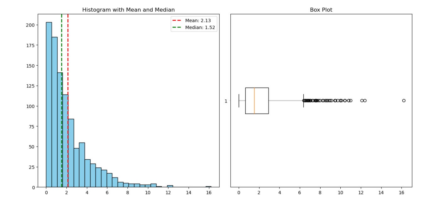
Histogram (left) and Boxplot (right) shows the distibution of the data which is skewed
For example, in the dataset represneted in figure above, which is skewed, the mean is affected by the outlier data points and is therefore higher than the median. In contrast, if the data distribution is approximately symmetrical, the mean and median would be relatively close to one another.
Measuring variability
Measures of central tendency alone are insufficient for fully understanding the shape of a dataset. Measures of variability provide insights into the spread or dispersion of the data points.
Range: The range of a dataset is calculated by subtracting the smallest value from the largest value within that dataset.
Interquartile Range (IQR): The interquartile range (IQR) represents the range of the middle 50% of a dataset. It is determined by subtracting the first quartile (25th percentile) from the third quartile (75th percentile). Because the IQR is less affected by outliers compared to the range, it is commonly used to summarize skewed data distributions.
Standard deviation: The standard deviation measures how far, on average, each data point is from the mean of the dataset, effectively quantifying the variability of a process. Unlike the range, which only considers the maximum and minimum values, the standard deviation takes into account the contribution of every value in the dataset to the overall dispersion, making it a more comprehensive measure of variability. Additionally, because it shares the same units as the original data, it is easier to interpret in context. The variance is simply the square of the standard deviation.
Introducing populations and samples
Statistics is the art of extracting meaningful insights from data, and it all begins with a thorough understanding of populations and samples.
Defining populations and samples
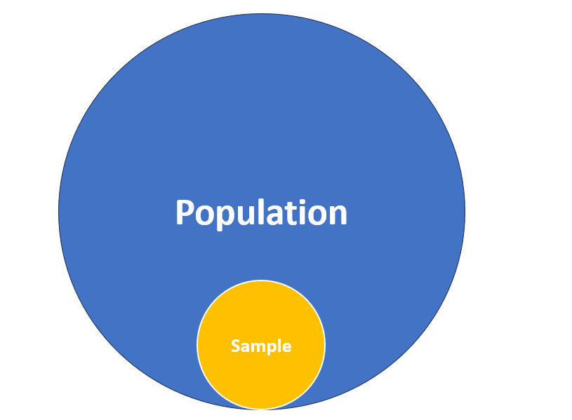
In the realm of statistics, a population refers to the entire group of individuals, objects, or events that we are interested in studying. For instance, if we wanted to research the average height of all adults in a country, the population would comprise every adult within that country. It would not include other countries or children, for example.
However, studying an entire population is often impractical or impossible due to factors such as time, cost, or accessibility. A sample is a subset of the population that we select to represent the larger group. By randomly selecting and analyzing a sample, we can draw meaningful conclusions about the population as a whole. In data science, we are almost always working on a dataset that represents the sample of a larger population.
Representing samples
The key to reliable statistical analysis lies in the representativeness of the sample. A representative sample accurately reflects the characteristics and diversity of the population it is drawn from. Achieving representativeness requires carefully considering factors such as sampling methods, sample size, and potential biases.
Simple random sampling is one of the most straightforward methods of sampling, where every individual in the population has an equal chance of being selected. This approach ensures that the sample is unbiased and, therefore, representative of the population, provided the sample size is sufficiently large.
Sampling bias occurs when we do not acquire a representative sample. It is a sample that is systematically skewed and does not accurately represent the population. In data science, it is essential to be aware of various sources of bias, such as selection bias, non-response bias, and measurement bias, to minimize their impact on statistical analysis and predictions.
Reducing the sampling error
When you take repeated samples from the same population, the results can vary due to natural fluctuations inherent in the data. Some of this variation may simply reflect these natural differences, while other discrepancies could indicate potential errors in the sampling process. The sampling error, often referred to as the standard error of a sample, represents the natural variation that occurs between different samples from the same population. This concept serves as a reminder that the estimates derived from our samples are not exact representations of the true population proportion, and that uncertainty and variability are always present in statistical analysis.
To mitigate the impact of the sampling error, we can increase the sample size and number of samples. The standard error is calculated as the standard deviation of the population statistic divided by the square root of the sample size.

SE is the standard error
sigma is the standard devaition of the population statistic
square root of n is the sample size
As the sample size grows larger, the stardard error decreases. Similarly, increasing the number of samples also reduces the sampling error. The more samples you collect, the better you can estimate the true population parameter by considering the range and distribution of estimates across the samples. To calculate the overall standard error when combining results from multiple samples, you can compute the standard deviation of the sample statistics across all the samples and divide it by the square root of the total number of samples. This accounts for the variability between the sample estimates.
Understanding the Central Limit Thereom (CLT)
The CLT states that regardless of the original population distribution’s shape, when we repeatedly take samples from that population and each sample is sufficiently large, the distribution of the sample means will approximate a normal distribution. This approximation becomes more accurate as the size of each sample becomes larger. This theorem plays a crucial role in measuring centrality by allowing us to make reliable estimates using these measures. In turn, the CLT enables us to estimate the population mean with greater accuracy, making the mean a powerful tool for summarizing data. It also indirectly influences the estimation of the median and mode. As the sample size increases, the distribution of individual observations becomes less skewed, enhancing the reliability of the median and mode as a measure of centrality.
The CLT also allows us to accept the assumption of normality, which allows us to rely on the normal distribution of sample means, even when the population distribution is not normal. Many statistical techniques and tests rely on the assumption of normality to ensure the validity of the inferences made. When the population follows a normal distribution, the CLT enables us to make accurate inferences about population parameters using sample means. This assumption allows us to use parametric tests.
Many parametric hypothesis tests (such as t-tests and z-tests) rely on the assumption of normality to make valid inferences. These tests assume that the population from which the sample is drawn follows a normal distribution. The CLT comes into play by allowing us to approximate the distribution of the test statistic to a normal distribution, even when the population distribution is not strictly normal. This approximation enables us to perform these tests and make reliable conclusions.
Demonstrating the assumption of normality
Let’s conduct an experiment where we roll a die repeatedly. We will be using a fair six-sided die, meaning that the die has not been altered, and there is an equal chance that when rolled, it might land on any of its six values. Since there is an equal chance of rolling any of the values on the die, this is considered a uniform distribution. In our experiment, we will repeatedly roll five times. Every time we roll the dice five times, we take the mean of our five die rolls. This is considered a sample. We repeat this process 10 times, computing 10 means:
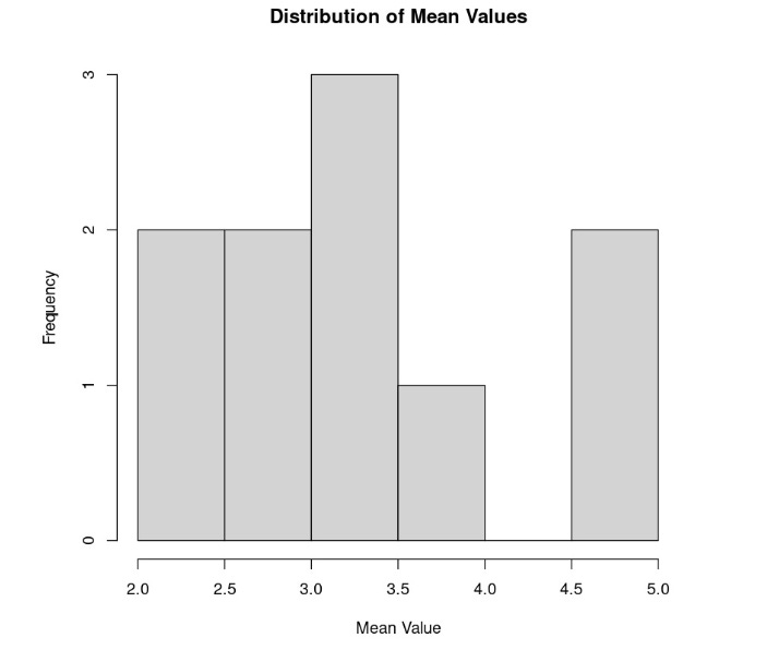
Now, let’s perform the same exercise, but this time, we’ll replicate the experiment 100 times (resulting in 100 samples) instead of 10:
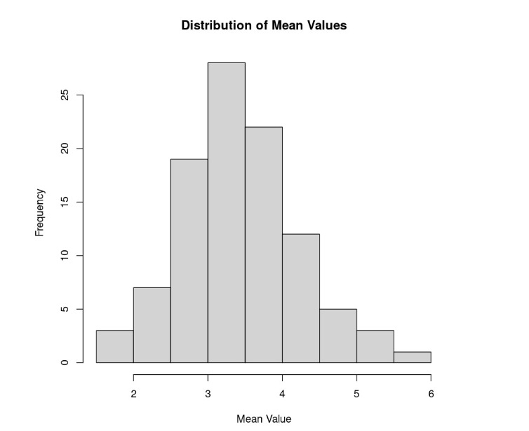
Lastly, let’s repeat the experiment one more time, only with 10,000 samples instead of 100:
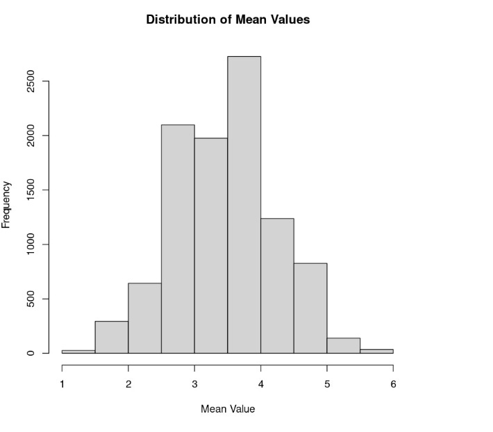
Notice that the sample mean distribution now resembles a normal distribution, even though we know that rolling dice theoretically fits uniform distribution. This illustrates the CLT – if you take a sufficiently large sample of random items from a population (typically 30 or more), regardless of the shape of the distribution of those items (as in our example of a uniform distribution from the die), the average of those samples will tend to approximate a normal distribution. This approximation becomes more accurate with larger sample sizes.
In terms of centrality, the CLT is primarily concerned with the mean. It asserts that with increasing sample sizes, the sample means tend to form a normal distribution, even if the original population distribution is not normal. This characteristic enhances the reliability and significance of the sample mean as a measure of central tendency, especially in making inferences about the population mean. However, the CLT does not directly impact the reliability of other centrality measures such as the median and mode, which depend on different aspects of the data distribution.
Shaping data with sampling distributions
Theoretical distributions describe a variable's central tendency and variability, guiding the choice of distribution for different data contexts, especially in data science.
Probability distributions
Probability distributions are fundamental concepts in statistics and probability theory that describe the likelihood of various outcomes in a random experiment or process. In the world of data science, these distributions play a crucial role in modeling and understanding uncertainty. By studying the properties and characteristics of different probability distributions, we can gain insights into real-world phenomena, make predictions, and perform statistical inference.
In data science, probability distributions represent the “shapes of data” for discrete and continuous variables, helping to visualize and analyze datasets. Discrete variables take on whole numbers, while continuous variables can hold any value within a range. Understanding a variable's distribution allows you to calculate probabilities and select appropriate models based on data assumptions.
Uniform distribution
The uniform distribution represents outcomes where each value within a given range is equally likely. Uniform distribution is frequently used in simulations and bootstrapping methods. It’s also the foundational building block for generating random numbers in algorithms and models.
Normal and student’s t-distributions
The normal distribution, also known as the Gaussian or Z distribution, is perhaps the most widely used and essential probability distribution. It is characterized by its bell-shaped curve and is completely determined by its mean (µ) and standard deviation (σ).
The z-score is a standardized value that measures how many standard deviations a given data point is from the mean.
The t-distribution is the normal distribution’s “cousin.” The biggest difference is that it’s generally shorter and has fatter tails. It is used instead of the normal distribution when the sample sizes are small. In t-distributions, the values are more likely to fall further from the mean. One thing to note is that as the sample size increases, the t-distribution converges to the normal distribution.
Binomial distribution
The binomial distribution models the number of successes in a fixed number of independent Bernoulli trials. A Bernoulli trial is a random experiment with two possible outcomes.
As a data scientist, it is important to remember that when using the binomial distribution, the probability of each success must also be the same for each trial. Also, there can only be two possible outcomes (hence “bi”) for each of the trials. Finally, you cannot use a binomial distribution if the trials are not independent.
Poisson distribution
Poisson distribution is the probability of a given number of (discrete) independent events happening in a fixed interval of time, and is commonly used in queuing theory, which answers questions like “How many customers are likely to purchase tickets within the first hour of announcing a concert?” These events must occur with a known constant mean rate and are independent of the time since the last event.
Each event must be independent of the others.
These must be discrete events, meaning that events occur one at a time.
It is assumed that the average rate of occurrences, 𝜆, is constant over the time interval.
Exponential distribution
Similar to the Poisson distribution, the exponential distribution is a continuous distribution that simply models the interval of time between two events. You can also think of this as the probability of time between Poisson events. The exponential distribution models the time between consecutive events in a Poisson process, where events occur at a constant average rate (𝜆). It is often used to model waiting times and lifetimes of certain processes. For example, the time between consecutive visits to a website follows an exponential distribution with an average rate of 0.1 visits per minute. This distribution assumes that the events occur at a constant rate and that each event is independent of each other.
Geometric distribution
The geometric distribution models the number of independent Bernoulli trials needed before observing the first success. Similar to the binomial distribution, we assume that each trial has two possible outcomes (success or failure), is independent of the others, and that the probability of success is the same for each trial. However, remember that the binomial distribution looks to model the number of successes over a fixed number of trials, while the geometric distribution models the number of trials required to achieve the first successful trial.
Weibull distribution
The Weibull distribution is a versatile distribution that’s used in reliability engineering and survival analysis. It can model various shapes, including exponential (special case) and bathtub curves. Weibull distribution is useful because of its flexibility, which is afforded to this distribution by two parameters: scale (𝜆) and shape (k). More specifically, the Weibull distributions are often used to model the time until a given technical device fails, but it also has other applications.
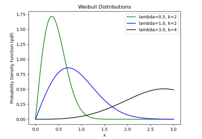
k=1 assumes constant failure rate which is essentially an exponential distribution. If k < 1 then it is a decreasing failure rate while k > 1 is increasing failure rate