Time Series Analysis and Forecasting Basics

Analysis of Sequential Data: Principles, Techniques, and Modern Approaches

Introduction to Time Series

Time series analysis is a fundamental concept in data science and statistics that deals with data points collected or recorded sequentially over time. Unlike regular regression problems, time series data has unique characteristics that require specialized analytical approaches.

What Makes Time Series Special?

1. Temporal Dependency: Each observation is dependent on previous observations

2. Fixed Time Intervals: Data is collected at consistent intervals (hourly, daily, monthly, etc.)

3. Natural Ordering: Data points follow a chronological sequence

4. Pattern Recognition: Often exhibits patterns like trends and seasonality

Core Components of Time Series

1. Trend

• Definition: The long-term movement or direction in the data

• Types:

  • Upward (increasing trend)

  • Downward (decreasing trend)

  • Horizontal (stable trend)

• Characteristics:

  • Can be linear or non-linear

  • Represents the general direction of the series

  • May change direction over time

2. Seasonality

• Definition: Regular and predictable patterns that repeat at fixed intervals

• Examples:

  • Retail sales increasing during holidays

  • Ice cream consumption peaking in summer

  • Weekly patterns in website traffic

• Characteristics:

  • Fixed and known frequency

  • Regular periodic fluctuations

  • Can be removed or adjusted for analysis

3. Cyclic Patterns

• Definition: Rises and falls without fixed frequency

• Difference from Seasonality:

  • Longer duration (usually >1 year)

  • Variable period length

  • Less predictable

• Examples:

  • Business cycles

  • Economic boom-bust cycles

  • Population cycles in ecology

4. Random Variation (Noise)

• Definition: Unpredictable fluctuations in the data

• Characteristics:

  • No discernible pattern

  • Can mask underlying patterns

  • Important for statistical modeling

Understanding Stationarity

What is Stationarity?

A time series is considered stationary when its statistical properties remain constant over time.

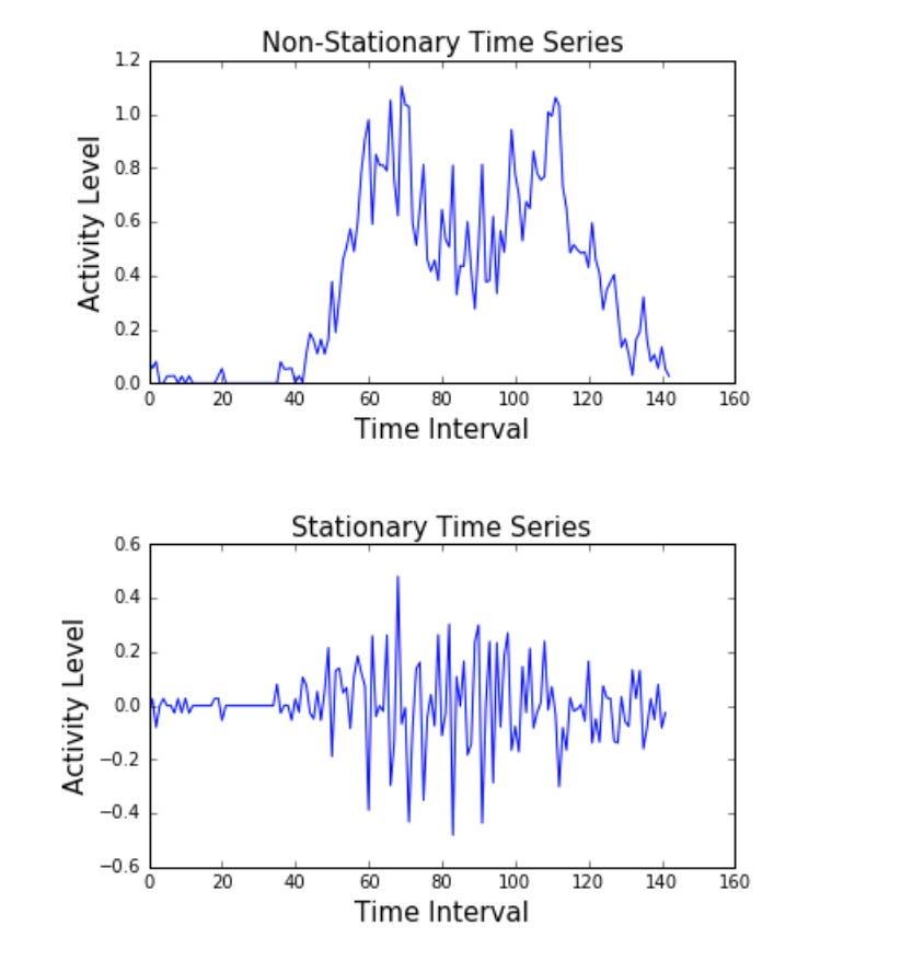
Stationary and Non-Stationary examples. Statistical properties are not constant for the Non-Stationary plot overtime.

Key Properties of Stationary Series:

1. Constant Mean: The average value stays consistent

2. Constant Variance: The spread of data remains stable

3. Constant Autocorrelation: The relationship between observations and their lagged values remains consistent

Testing for Stationarity

1. Visual Inspection

• Plot the time series

• Look for obvious trends

• Check for changing variance

• Examine seasonal patterns

2. Statistical Tests

1. Augmented Dickey-Fuller (ADF) Test

   • Null hypothesis: Series is non-stationary

   • Alternative hypothesis: Series is stationary

   • Decision rule: Reject null if test statistic < critical value

2. KPSS Test

   • Complements ADF test

   • Tests for trend stationarity

   • Often used in conjunction with ADF

3. Phillips-Perron (PP) Test

   • Similar to ADF

   • More robust to unspecified autocorrelation

Making Time Series Stationary

Methods:

1. Differencing

   • First difference: Yt - Yt-1

   • Second difference: (Yt - Yt-1) - (Yt-1 - Yt-2)

   • Continue until stationary

2. Mathematical Transformations

   • Logarithmic transformation

   • Square root transformation

   • Box-Cox transformation

3. Decomposition

   • Separate trend

   • Remove seasonality

   • Analyze residuals

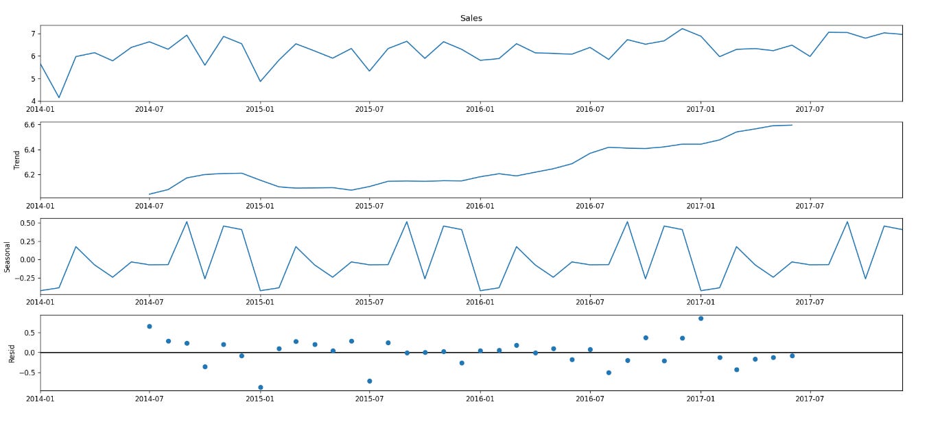
Decomposition

Example of Differencing:

Original series: [1, 5, 2, 12, 20]

• First difference: [4, -3, 10, 8]

• Second difference: [-7, 13, -2]

Time Series Forecasting Methods

1. Classical Methods

• Moving Averages

• Exponential Smoothing

• SARIMA Models

2. Modern Approaches

• Neural Networks

• Deep Learning Models

• Prophet (Facebook)

• LSTM Networks

Best Practices for Time Series Analysis

1. Data Preparation

   • Handle missing values

   • Check for outliers

   • Ensure consistent time intervals

2. Pattern Identification

   • Decompose series

   • Identify seasonal patterns

   • Detect trends

3. Model Selection

   • Consider data characteristics

   • Evaluate multiple models

   • Use appropriate error metrics

4. Validation

   • Use time-based cross-validation

   • Consider forecast horizon

   • Account for seasonality in validation

Common Applications

1. Financial forecasting

2. Sales prediction

3. Weather forecasting

4. Population growth analysis

5. Economic indicators

6. Energy consumption prediction

7. Website traffic analysis

Performance Metrics

1. Mean Absolute Error (MAE)

2. Mean Squared Error (MSE)

3. Root Mean Squared Error (RMSE)

4. Mean Absolute Percentage Error (MAPE)

5. Theil's U Statistics

Conclusion

Time series analysis is a powerful tool for understanding and predicting patterns in temporal data. Success in time series analysis requires:

• Understanding of core concepts

• Proper data preparation

• Appropriate model selection

• Rigorous validation

• Regular model updating and maintenance