Understanding Backpropagation: The Heart of Neural Network Learning

How Gradients, Chain Rule, and Gradient Descent Power Neural Networks to Improve Predictions and Mathematics behind it

Backpropagation is the core mechanism by which neural networks learn and improve over time. It works by iteratively updating the model's weights and biases to minimize the error (or loss) between the predicted output and the true label. This process involves computing gradients of the loss function with respect to each parameter, typically using the chain rule from calculus.

However, as neural networks become more complex (with many layers and large amounts of data), the process of backpropagation becomes computationally intensive. This is where modern hardware, like GPUs, and vectorization techniques play a crucial role.

Iterative Nature of Backpropagation

Backpropagation is an iterative process, meaning that it repeats over multiple steps or epochs to gradually adjust the weights and biases. Here’s how the iterative nature works:

1. Forward Pass: Initially, a forward pass is made through the network where the input data is propagated through each layer, calculating activations until reaching the output layer. This provides the predicted output.

2. Compute Loss: The difference between the predicted output and the true label is then measured using a cost function, like cross-entropy loss for classification problems.

3. Backward Pass (Backpropagation): In the backward pass, gradients are computed layer by layer, starting from the output layer and moving backward toward the input layer. At each layer, the gradients (partial derivatives) are calculated using the chain rule of calculus. These gradients indicate how much each weight or bias needs to be adjusted to reduce the cost function.

4. Gradient Descent: The gradients are then used to update the weights and biases via an optimization algorithm like stochastic gradient descent (SGD) or Adam. This step adjusts the model's parameters to minimize the loss. The process is repeated across multiple iterations or epochs until the model converges to an optimal set of parameters.

Role of GPUs in Backpropagation

In deep learning, especially when training large models with millions of parameters, performing these calculations using traditional CPU-based systems can be very slow. GPUs (Graphics Processing Units) have become crucial in speeding up the process of training neural networks. Here's why:

1. Parallel Processing: GPUs are designed for parallel processing, meaning they can perform many operations simultaneously. Neural networks, particularly deep ones, involve massive matrix operations (like multiplications and additions). Since these operations can be done independently across different neurons and layers, GPUs excel in performing them efficiently in parallel.

2. Faster Computations: With thousands of cores dedicated to executing tasks simultaneously, GPUs can handle much more data and perform more calculations per second than CPUs, making backpropagation and other steps in the training process much faster.

3. Handling Large Datasets: Deep learning models often require the processing of large datasets. With GPUs, these large volumes of data can be processed in a fraction of the time it would take using CPUs, allowing for faster training and experimentation.

Vectorization: Optimizing Computations

Vectorization refers to the process of converting operations that would normally be executed in a loop into vectorized operations, which can be computed all at once. This is a critical optimization technique for neural networks because:

1. Efficiency: Instead of processing individual elements of a matrix or vector one at a time, vectorization allows the entire matrix or vector to be processed in parallel. This takes full advantage of the capabilities of modern processors (especially GPUs).

2. Optimization Libraries: Libraries like NumPy, TensorFlow, and PyTorch leverage vectorization to perform matrix multiplications, element-wise operations, and other calculations much more efficiently. They use low-level optimizations to ensure that these operations run quickly and scale across different hardware platforms.

3. Backpropagation Example: During the backpropagation step, we compute gradients for the weights and biases in a neural network. If done naively using loops, this would be computationally expensive. However, by using vectorized operations, we can compute the gradients for all weights and biases in parallel, significantly reducing the time required for this step.

Iterative Process and Convergence

Backpropagation, as mentioned, is an iterative process, and the gradients are computed multiple times over many epochs. The model starts with random weights and biases, and each pass of backpropagation refines the parameters:

1. Epochs and Mini-batches: During training, the dataset is often split into mini-batches, and backpropagation is performed on each mini-batch. This is known as mini-batch gradient descent, and it helps reduce computational costs compared to calculating gradients on the entire dataset.

2. Convergence: Over successive iterations, the model’s weights and biases converge to values that minimize the cost function. The goal of training is to reach a point where the gradients are close to zero (indicating that the network is not making large changes) and the cost function is at a minimum.

3. Learning Rate: The learning rate determines how much the weights are adjusted in each step. If the learning rate is too large, the model may overshoot the optimal solution; if it's too small, the training may take too long.

Mathematics behind Backpropagation

To grasp the mathematics behind this algorithm, let’s consider a simple example:

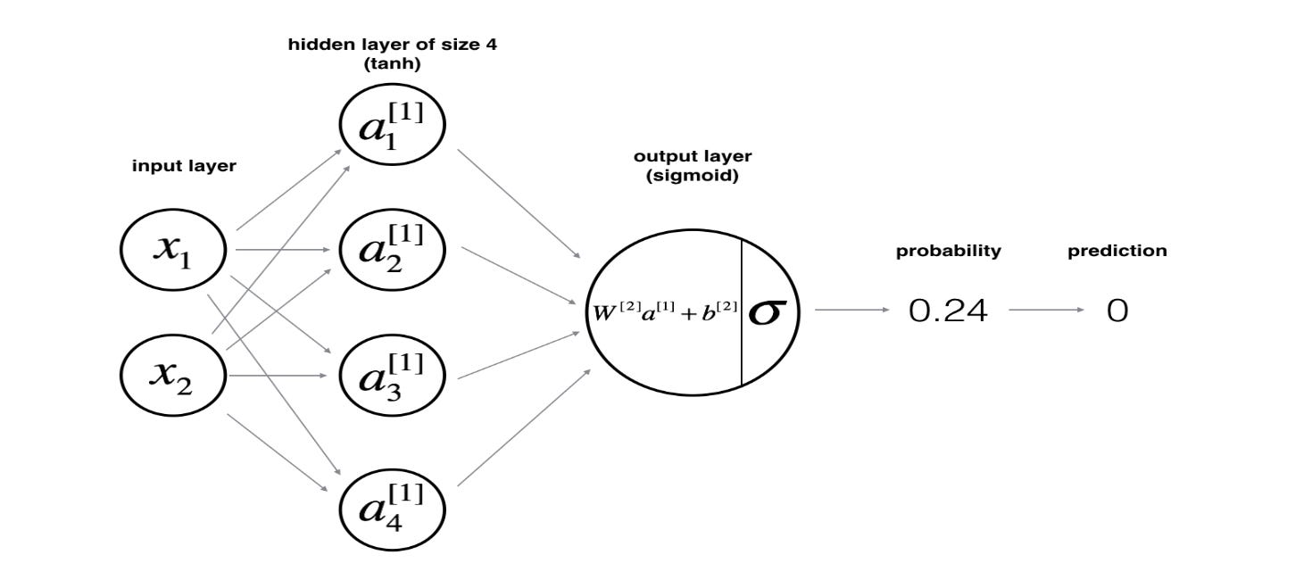
In the diagram above:

• Two input features, x1 and x2 feed into four hidden units.

• Each hidden unit computes an intermediate activation using the tanh function.

• The output layer combines these hidden activations using learned weights and bias, and passes the result through a sigmoid function to output a probability.

• The prediction is compared with the true label using a cost function (e.g., cross-entropy loss), which measures how far off our guess is.

Forward Pass

We can write the mathematical form of the output prediction as:

\(a = \sigma\left(W^{[2]} a^{[1]} + b^{[2]}\right) \)

Where:

• a[1] is the vector of activations from the hidden layer

• W[2], b[2] are the weight and bias of the output layer

• σ is the sigmoid activation function

• a is the final predicted probability

The cost function is then:

\(J = -\left[y \log(a) + (1 - y) \log(1 - a)\right] \)

The cost function above is also referred to as cross entropy loss function.

Backward Pass

To train the network, we want to adjust the weights and biases to reduce the cost function. This is where backpropagation comes in!

The Chain Rule Behind the Scenes

Backpropagation works by applying the Chain Rule from calculus. It helps us trace how a small change in the final prediction affects earlier layers by breaking down the total derivative into manageable parts.

The key mathematical principle that makes backpropagation work is the Chain Rule of Calculus. It allows us to compute the derivative of a function that depends on other functions by linking the rates of change across them. In simple terms, it helps us understand how a change in one quantity affects another when they are connected through multiple steps.

In deep neural networks, which may contain hundreds of such steps across many layers, applying the chain rule repeatedly becomes computationally intensive. This is where modern hardware like GPUs and optimized techniques like vectorization make training feasible by handling millions of derivative calculations efficiently.

Gradients in the Output Layer

We begin by computing how the cost changes with respect to the output:

\(\frac{\partial a}{\partial J} = -\left( \frac{a}{y} - \frac{1 - a}{1 - y} \right) \)

Then, we move backward to find how the cost changes with respect to the weighted input:

where:

\(z^{[2]} = W^{[2]} a^{[1]} + b^{[2]} \)

Gradients in the Hidden Layer

To compute the gradients for W^[2] and b^[2] :

\(\frac{\partial J}{\partial W^{[2]}} = \frac{\partial J}{\partial z^{[2]}} \cdot (a^{[1]})^T \)

\(\frac{\partial J}{\partial b^{[2]}} = \frac{\partial J}{\partial z^{[2]}} \)

We repeat the chain rule to move backward to the previous layer:

\(\frac{\partial J}{da^{[1]}} = (W^{[2]})^T \cdot \frac{\partial J}{\partial z^{[2]}}\)

\(\frac{\partial J}{\partial z^{[1]}} = \frac{\partial J}{\partial a^{[1]}} \cdot \tanh'(z^{[1]})\)

And then finally compute:

\(\frac{\partial J}{\partial W^{[1]}} = \frac{\partial J}{\partial z^{[1]}} \cdot X^T \)

\(\frac{\partial J}{\partial b^{[1]}} = \frac{\partial J}{\partial z^{[1]}} \)

This process is repeated for each training example in the dataset. The gradients are computed layer by layer, and the weights and biases are adjusted accordingly. This is done for multiple iterations (or epochs) until the weights and biases converge to values that minimize the cost function. The process of updating the weights using the gradients is known as gradient descent!

As the weights and biases are fine-tuned through these updates, the model becomes better at making predictions and minimizing errors, enabling it to generalize better to unseen data.

This is the backbone of neural network learning. By efficiently computing these gradients for each layer, we can update the parameters using gradient descent to minimize the loss function.

Modern deep learning frameworks like TensorFlow and PyTorch automate this process. However, understanding the mechanics of backpropagation helps demystify what's going on under the hood.

As can be seen, backpropagation is the core mechanism that makes learning possible in neural networks, enabling them to continuously improve and adapt through multiple iterations.