


In this post, I’ll explore Variational Autoencoders (VAEs) is often compared to Generative Adversarial Networks (GANs) but follow a fundamentally different approach. Alongside the conceptual overview, I’ll demonstrate a VAE implementation using the MNIST dataset. Unlike my previous post on GANs, this time I’ll begin with a high-level explanation of discriminative vs. generative models to provide better context for understanding VAEs.
In machine learning, models generally fall into two broad categories: discriminative and generative.
Discriminative models focus on learning the decision boundary between classes. They model P(y∣x), the probability of a label given the input. Examples include logistic regression, decision trees, and most supervised deep learning models.
Generative models, on the other hand, aim to model the data generation process itself. They try to learn P(x) or P(x,y), and can generate new samples that resemble the training data. Examples include Naive Bayes, GANs, and VAEs.
While discriminative models are generally more accurate for classification given enough labeled data, generative models are more flexible and powerful in scenarios like semi-supervised learning, unsupervised learning, and data generation.
Generative models can be turned into a classifier (essentially what the LLM like ChatGPT does!) using Bayes Rule:
However, this process often becomes complex and intractable especially in high dimensional spaces.
Generative models typically make stronger assumptions about the data distribution than their discriminative counterparts. As a result, they often suffer from higher asymptotic bias. This means that even with more data, their bias may not decrease if those assumptions are incorrect. In contrast, discriminative models, which make fewer assumptions, can often achieve better performance as the dataset grows, since they directly model the decision boundary. As a general rule of thumb:
When there is a large amount of labeled data, discriminative models generally perform well.
When labeled data is limited, such as in semi-supervised learning, it can be beneficial to use a generative model to guide or regularize the training of a discriminative model.
What is VAE?
Variational Autoencoders (VAEs) are a class of generative models that blend deep learning with probabilistic inference. Unlike traditional autoencoders that compress data into deterministic latent vectors, VAEs model a distribution over the latent space. That means the latent space is treated as a set of random variables. Specifically, VAE assumes that each input x is generated from some latent variable z, and z~p(z), typically a standard normal distribution. Instead of learning a fixed point in latent space for each input, VAEs learn a distribution, that is, q(z|x) which reflects uncertainty in the latent.
This gives VAEs several advantages:
They can generate new data by sampling from the latent space.
They learn meaningful latent representations, which can be used for clustering, interpolation, and downstream tasks.
They are fully differentiable, allowing training via stochastic gradient descent.
A VAE consists of two main components:
Encoder (Inference Network)
Learns to map input data x to a distribution over latent variables z, i.e., q(z∣x). This is often modeled as a Gaussian with parameters μ(x),σ(x).Decoder (Generative Network)
Maps latent variables z back to the data space to reconstruct x, i.e., it models p(x∣z).
These two components are optimized jointly using variational inference, specifically maximizing the Evidence Lower Bound (ELBO):
The first term encourages accurate reconstruction.
The second term (KL divergence) ensures that the learned latent distribution stays close to the prior (often standard normal).
Kullback-Leibler (KL) divergence is a key concept in information theory and a core component of VAE loss function. It measures how much one probability function diverges from the second expected distribution. KL Divergence regularizes the latent space by keeping q(z|x) close to p(z).
Moreover, since the encoder does not produce a single vector but rather the parameters of a distribution (mean and variance), during training, it is usually sampled z from this distribution using reparameterization trick, which allows gradients to flow through a sampling step:
This stochastically forces the model to learn robust, smooth, and continuous representations.
To elaborate, it is worth noting that the reparameterization trick is not unique to VAEs. It is commonly used in Bayesian deep learning to enable gradient-based optimization when sampling from probability distributions. In Bayesian models, to optimize over a distribution (posterior over latent variables), sampling from the distribution introduces non-differentiable operations making gradient based optimization difficult.
The reparameterization trick addresses the challenge of non-differentiability in sampling by rewriting the sampling operation in a differentiable form. This enables gradient-based optimization in models like the Variational Autoencoder.
Choosing the simpler and tractable family of distributions (called variational family) to approximate the true posterior.
Optimizing the parameters to make this variational distribution as close as possible to true posterior distribution, usually by minimizing the KL divergence between them.
Instead of computing the exact posterior, VI maximizes the Evidence Lower Bound (ELBO), which provides a tractable objective as described above.
I implemented a VAE on the MNIST dataset using PyTorch to demonstrate variational inference in practice. Since VAEs are highly flexible and depend on the nature of the data and modeling choices, there's no fixed API. Instead, the architecture is typically built manually, including encoder, decoder and loss function.
Here are some important components to note:
class VAE(nn.Module):
    def __init__(self, latent_dim = 20):
        super(VAE, self).__init__()
        self.fc1 = nn.Linear(28*28, 400)
        self.fc_mu = nn.Linear(400, latent_dim)   # from 400 dim hidden vector to compute mean of latent space
        self.fc_logvar = nn.Linear(400, latent_dim) # from 400 dim hidden vector to compute log variance of latent space
        self.fc_dec = nn.Linear(latent_dim, 400) # maps the latent vector z back to the hidden space
        self.fc_out = nn.Linear(400, 28*28) # reconstructs the input image from the hidden space

def encode(self, x):
        h1 = F.relu(self.fc1(x))
        return self.fc_mu(h1), self.fc_logvar(h1)  # returns mean and log variance of the latent space


def decode(self, z):
        h2 = F.relu(self.fc_dec(z))
        return torch.sigmoid(self.fc_out(h2))  # reconstruct the image with sigmoid activation

def reparameterize(self, mu, logvar):
        std = torch.exp(0.5 * logvar)
        eps = torch.randn_like(std)  # sample from standard normal dist
        return mu + eps * std  # reparameterization trick

def forward(self, x):
        mu, logvar = self.encode(x.view(-1, 28*28))  # flatten the input
        z = self.reparameterize(mu, logvar)  # sample the latent space
        x_recon = self.decode(z)  # reconstruct the image
        return x_recon, mu, logvar  # return reconstructed image


def vae_loss(recon_x, x, mu, logvar):
    BCE = F.binary_cross_entropy(recon_x, x.view(-1, 28*28), reduction='sum')  # Binary Cross Entropy loss
    KLD = -0.5 * torch.sum(1 + logvar - mu.pow(2) - logvar.exp())  # Kullback-Leibler divergence
    return BCE + KLD  # return total loss
Inherits the neural network class from pytorch. Initializes the network with latent_dim. latent_dim is the dimension of the latent variable z which is usually a small vector to capture features of the image.
The first layer of encoder takes in flattened 28*28 image and maps to a hidden layer of 400. choice of 400 is arbitrary - as from deep learning literature, too high might lead to overfitting while too low may not capture the inherent relationship efficiently. Then, activation function typically ReLU is applied. The first layer acts as a shared base.
In the second stage of the encoder, the network computes the mean and log-variance vectors from the 400-dimensional hidden representation. These vectors define the parameters of the latent Gaussian distribution used for sampling.
Next, a latent vector is sampled using reparameterization trick. The reparameterize function enables differentiable sampling from a Gaussian distribution by expressing the latent variable z as a deterministic transformation of the mean, log-variance, and random noise. This is essential for training VAEs using gradient-based optimization. First, it converts the log-variance to standard deviation. Then it samples the standard normal noise. Then it reparameterizes the latent variable using the equation described earlier in the post.
The final decoder layer converts the latent variable z to 400D hidden layer. The hidden layer is then mapped back to the original input shape after applying activation function to convert back to pixel.
The loss function that combines reconstruction loss and KL divergence is used as to optimize the network where the model is trained for x number of epochs to minimize the loss and learn meaningful representations.
Finally, here is what the result looks like:
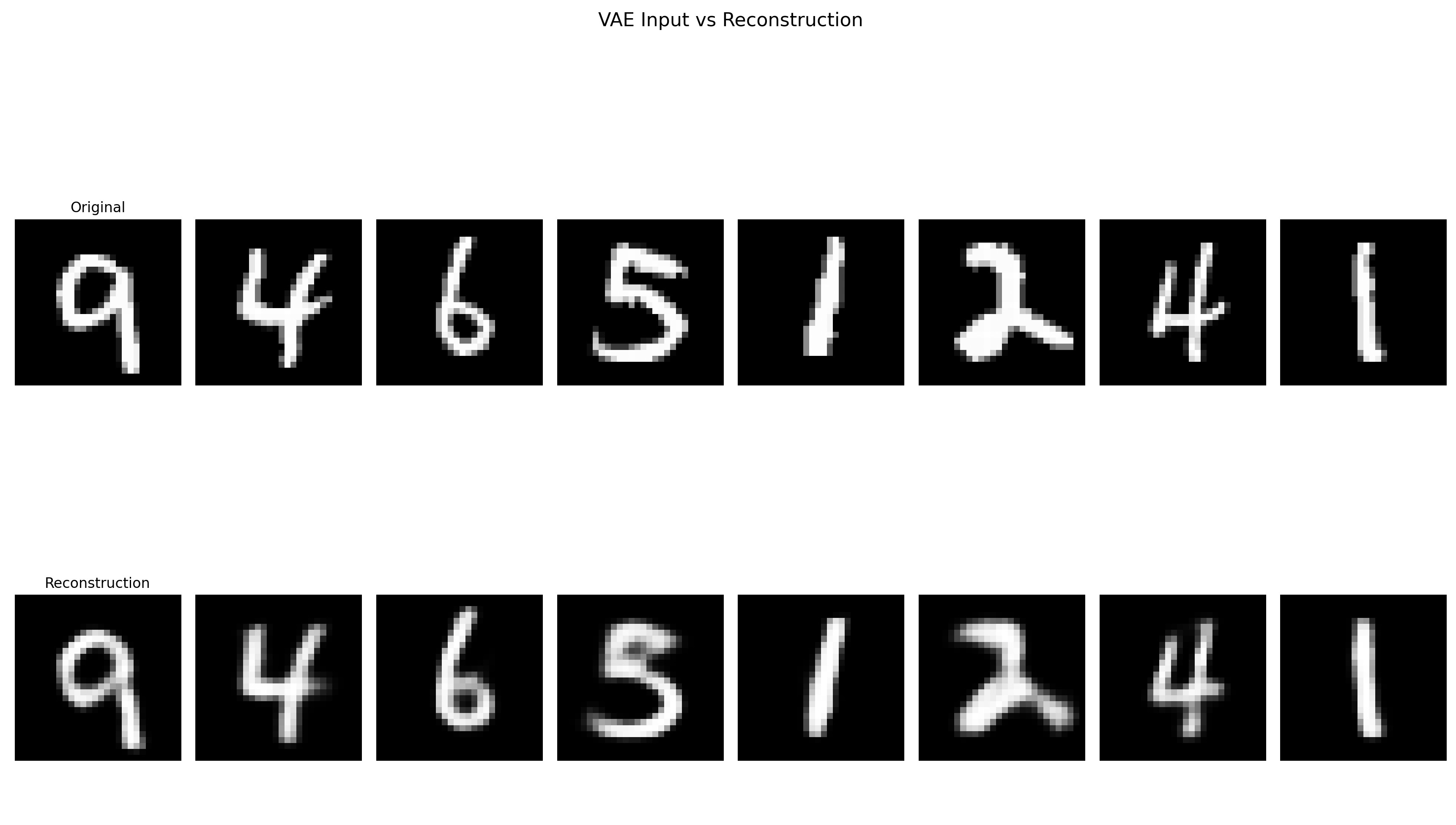
Two things to note
First, this model was only trained for a few epochs using a simple architecture with no tuning, so the image quality can certainly be improved with more training and better hyperparameter choices.
Second, and more importantly, it is a well-known observation that the images generated by VAEs tend to be slightly blurry compared to those produced by GANs. This happens because VAEs optimize a reconstruction loss, which encourages the model to produce an average over possible outputs. This averaging effect often results in smoother but less sharp images.
In contrast, as discussed in a previous post, GANs use a discriminator to guide the generator toward producing images that are indistinguishable from real ones. This adversarial training setup encourages sharper and more realistic results but often comes with training instability and less interpretability.
To address these trade-offs, several models have been proposed that combine the VAE and GAN frameworks. Examples include VAE-GAN, IntroVAE, and BicycleGAN, which aim to preserve the structured latent space of VAEs while enhancing image quality through adversarial training.